How AI Can Estimate Impermanent Loss in DeFi Liquidity Pools

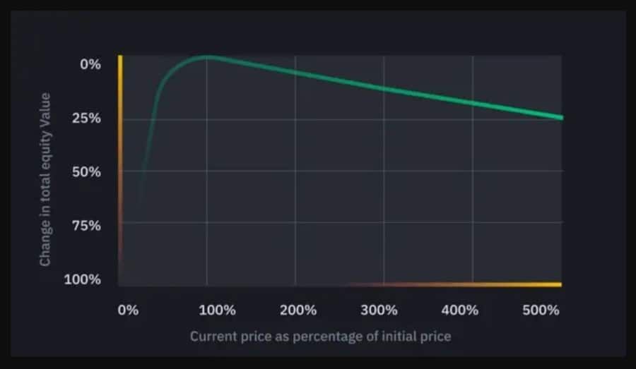
How AI Can Estimate Impermanent Loss

AI can estimate impermanent loss by modeling how a liquidity position changes when token prices move, then comparing that position with the value of simply holding the deposited assets. The model can improve the estimate by incorporating price volatility, trading fees, liquidity ranges, market conditions, and multiple possible future scenarios.

It cannot know the future price path with certainty. A useful AI estimate is therefore a range of potential outcomes, not a guaranteed prediction.

Impermanent loss occurs when the relative prices of tokens change after a liquidity provider deposits them into an automated market maker, or AMM. The provider may end up with a lower portfolio value than if the original tokens had remained in a wallet. Uniswap describes this comparison as a value difference caused by price changes from the time liquidity was added.Uniswap’s explanation of impermanent loss

The loss is called “impermanent” because it can shrink if prices return toward their original relationship. However, the loss is not automatically reversed, and withdrawing while prices remain different can make the result permanent.

Why Impermanent Loss Is Difficult to Estimate

A simple calculation can estimate loss from an initial price ratio and a final price ratio. Real liquidity positions are more complicated because the result depends on several interacting variables:

The relative price change between the two assets.
The time spent at different prices.
The pool’s pricing formula.
The amount of liquidity competing in the pool.
Trading fees earned during the position’s lifetime.
Whether liquidity is active across the current price.
Rebalancing, deposits, withdrawals, and compounding.
Network fees, execution costs, and possible failed transactions.
Smart-contract, oracle, and market-manipulation risks.

For a basic constant-product pool, Uniswap’s developer documentation gives a standard impermanent-loss calculation based on the change in the token price ratio.Uniswap’s returns documentation The calculation is useful for a first estimate, but it does not describe the complete economic result. Fees and transaction costs must be evaluated separately.

Concentrated liquidity adds another challenge. In Uniswap v3, liquidity providers select a price range, and their liquidity is active only while the market price remains inside that range. Academic research on Uniswap v3 shows that the position’s composition and risk change as the price moves through the selected range.Research on Uniswap v3 liquidity-provider risk

What Data an AI Model Needs

An AI system should begin with a structured record of the liquidity position. Without reliable inputs, even a sophisticated model produces misleading output.

Position data

The model should know:

The pool and blockchain.
The deposited token amounts.
The deposit timestamp.
The deposit price ratio.
The withdrawal or evaluation date.
The selected lower and upper price bounds, if the pool uses concentrated liquidity.
Whether fees are collected, reinvested, or left unclaimed.
Any additional deposits or withdrawals.

A position-level model is more useful than a generic prediction for a token pair. Two providers can supply the same pool but face different outcomes because they entered at different prices or chose different ranges.

Market data

The model also needs historical and current market information:

Token prices at suitable time intervals.
Pool reserves or liquidity distribution.
Trading volume.
Fee rates.
Price impact and swap activity.
Prices from external venues for comparison.
Block timestamps and transaction data.

The data should be adjusted for token decimals, chain reorganizations, missing blocks, stale prices, and abnormal trades. A model trained on unclean data may treat a bad oracle update or a one-block price spike as a normal market movement.

On-chain position data

For concentrated-liquidity pools, the model should read the position’s actual liquidity, tick range, fee-growth variables, and current pool state. A position can be technically open but economically inactive if the current price has moved outside its range.

This distinction matters because a position outside its range may hold mostly one token and stop earning fees until the price returns. Treating all deposited liquidity as continuously active can materially understate risk.

The Main AI Approaches

AI can estimate impermanent loss in several ways. The best method depends on whether the goal is a quick scenario analysis, a probabilistic forecast, or a live monitoring system.

1. Supervised regression

A regression model learns relationships between market and position variables and a target such as:

Future impermanent loss after one day.
Future impermanent loss after one week.
Net return after fees.
Probability that the position loses more than a chosen threshold.
Expected time before a concentrated position leaves its range.

Inputs might include realized volatility, trading volume, price distance from the range boundaries, liquidity depth, and recent return patterns.

Models such as gradient-boosted trees can work well with structured tabular data. They are often easier to inspect than a large neural network because the model can show which variables influenced a forecast.

The weakness is distribution shift. A model trained during calm markets may perform poorly during a sudden depeg, exchange failure, exploit, or regulatory shock.

2. Time-series forecasting

A time-series model forecasts possible future prices or price ratios. The forecast can then feed into an impermanent-loss calculator.

This approach is useful when the model captures changing volatility rather than assuming that future returns resemble a single long-term average. However, forecasting the token price is not the same as forecasting liquidity-provider returns. Fees, range activity, and arbitrage behavior still need separate treatment.

A price model that predicts the average future price may be insufficient. Two paths can finish at the same price while producing different outcomes for a concentrated position. One path may remain inside the range and earn fees; another may leave the range early and remain inactive.

3. Monte Carlo scenario generation

Monte Carlo simulation generates many possible future price paths. For each path, the system calculates the position value, fees, and comparison with holding the original assets.

The output can include:

Median estimated loss.
Best and worst modeled outcomes.
A selected downside percentile.
Probability of leaving the range.
Probability that fees offset the modeled impermanent loss.
Expected net return after specified costs.

This approach is often more informative than a single-point prediction because it makes uncertainty visible. It also allows the model to test correlated and uncorrelated token behavior.

The scenarios must still be realistic. Randomly sampling historical returns may miss volatility clustering, jumps, liquidity gaps, and correlation breakdowns. A robust system should compare several assumptions rather than rely on one simulation design.

4. Machine-learning classification

A classifier can answer decision questions instead of predicting an exact loss:

Is the position likely to leave its range within seven days?
Is projected fee income likely to be insufficient under the selected scenario?
Is the pool showing an unusual divergence event?
Has current volatility entered a high-risk regime?

Classification can make alerts easier to use, but thresholds need careful calibration. An alert that fires too often becomes noise, while an alert that is too conservative may fail during rapidly changing conditions.

A Practical Estimation Workflow

A reliable workflow separates mechanical calculation from uncertain forecasting.

Step 1: Reconstruct the position

Start with the actual token amounts, entry ratio, range, liquidity, fees, and timestamps. Do not estimate from the current pool balance alone.

Step 2: Calculate the mechanical baseline

Compute the position’s value at several hypothetical price ratios. Compare each result with the value of holding the original token amounts.

This baseline answers a narrow question: what would happen if the price moved to a specified level, before forecasting whether that level is likely?

Step 3: Model the price ratio

Use historical price data to estimate volatility, correlations, jumps, and possible regimes. For a stablecoin pair, depeg scenarios may matter more than ordinary day-to-day volatility. For volatile assets, trend changes and correlation breakdowns may dominate.

Step 4: Simulate the position

For each generated price path, update the position as the price changes. A concentrated-liquidity model must determine when the position is active, when it becomes one-sided, and when it re-enters the selected range.

Step 5: Add fees carefully

Fee income should be modeled from expected trading activity, fee tiers, share of active liquidity, and the provider’s actual position. High volume does not automatically mean high earnings for every provider.

Fees can offset impermanent loss, but they are not guaranteed. They may fall when volatility or trading activity changes. Fee estimates should therefore be presented as scenarios rather than fixed income.

Step 6: Include implementation costs

Subtract gas costs, swap fees, rebalancing costs, bridge costs, and expected slippage. For smaller positions, these costs can dominate the difference between a theoretical and practical return.

Step 7: Report a distribution

A useful result might say:

The modeled median net outcome is a loss of a certain amount.
The position has a specified probability of leaving its range.
Fee income offsets the modeled loss in only some scenarios.
Results are highly sensitive to volatility and correlation assumptions.

The system should display assumptions beside every result.

Comparing Estimation Approaches

Approach	Best use	Main strength	Important limitation
Fixed-price scenario	Quick planning	Transparent and easy to audit	Does not estimate whether the price target will occur
Historical simulation	Initial risk review	Uses observed market behavior	Past conditions may not represent future shocks
Monte Carlo model	Range of possible outcomes	Shows uncertainty and tail scenarios	Results depend heavily on assumptions
Regression model	Repeated short-horizon forecasts	Can combine many structured variables	May fail when market conditions change
Hybrid monitoring system	Live position management	Combines mechanics, forecasts, and alerts	More data, maintenance, and validation are required

No method removes the underlying risk. A transparent baseline combined with scenario analysis is usually more useful than a complex model that hides its assumptions.

What AI Can Detect Better Than a Spreadsheet

A spreadsheet is often sufficient for a single price scenario. AI becomes more valuable when the number of pools, positions, and market conditions grows.

An AI monitoring system can:

Track many positions continuously.
Detect unusual volatility or volume changes.
Estimate the chance of crossing a range boundary.
Compare current conditions with historical regimes.
Recalculate outcomes after deposits, withdrawals, and fee claims.
Identify when model assumptions are no longer reliable.
Prioritize positions that need manual review.

These capabilities support risk management rather than automatic decision-making. The system can surface a deteriorating position, but a provider still needs to decide whether the expected fees justify the exposure and transaction costs.

The Difference Between Impermanent Loss and Net Return

Impermanent loss is not the same as total profit or loss. It compares providing liquidity with holding the original assets. Net return includes additional components:

Trading fees.
Token emissions or incentives.
Price appreciation or depreciation of the assets.
Gas and execution costs.
Rebalancing activity.
Borrowing costs, if leverage is used.
Taxes or reporting consequences, depending on jurisdiction.

A position can have negative impermanent loss but positive net return if fees and incentives are sufficiently large. It can also have modest impermanent loss but negative net return if volume is weak or operating costs are high.

Academic work on AMMs emphasizes that fee income, arbitrage, and market dynamics affect the economic result beyond a simple price-divergence calculation.Research on impermanent loss and loss-versus-rebalancing

Model Risks and Failure Modes

AI estimates can fail in predictable ways.

Bad or incomplete data

Missing swaps, inaccurate token prices, stale oracle values, and incorrect pool metadata can corrupt the forecast. Data validation should be treated as part of the model, not an afterthought.

Overfitting

A model may memorize patterns from a particular market period. Strong historical accuracy does not prove that the model will work during a new regime.

False precision

Reporting an estimate such as “the position will lose 3.27 percent” implies more certainty than the evidence supports. A range, confidence interval, or scenario distribution communicates risk more honestly.

Ignoring tail events

Stablecoin depegs, smart-contract exploits, oracle failures, chain outages, and sudden liquidity withdrawals can produce outcomes outside ordinary historical observations.

Confusing correlation with causation

High trading volume may coincide with high fee income, but it can also coincide with severe price moves and greater impermanent loss. The model should test whether a relationship persists after controlling for relevant variables.

Treating fees as guaranteed

Fee forecasts depend on future volume, competition, active liquidity, and pool design. They should be stress-tested rather than added as a fixed annual percentage.

How to Evaluate an AI Estimate

Before relying on an estimate, ask:

Is the position reconstructed from verified on-chain data?
Is the calculation comparing liquidity provision with holding?
Does it include the correct pool design and price range?
Are fees modeled separately from impermanent loss?
Are gas, slippage, and rebalancing costs included?
Does the model provide multiple scenarios?
Has it been tested on periods outside the training sample?
Does it report performance during volatile markets?
Can the assumptions and inputs be inspected?
Does it identify when the forecast is outside its reliable range?

A good system should allow a user to reproduce the mechanical calculation even if the predictive model is unavailable. Explainability is especially important when the estimate influences a financial decision.

A Simple Hypothetical Example

Consider a provider who deposits two volatile tokens into a concentrated-liquidity pool. The provider selects a narrow range around the current price.

An AI system could generate three broad scenarios:

In the stable scenario, the price remains inside the range, trading activity stays moderate, and fees accumulate steadily.
In the trending scenario, the price moves beyond the upper boundary, leaving the position mostly exposed to one token and reducing fee generation.
In the shock scenario, volatility rises sharply, the price crosses the range quickly, and estimated execution costs increase during rebalancing.

The model would calculate the position value under each path, compare it with holding the original tokens, add modeled fees, and subtract costs. The result would be a set of conditional outcomes, not a promise about what will happen.

This approach is more useful than asking AI for a single “safe” pool. Safety depends on the assets, range, time horizon, liquidity depth, smart-contract risk, and the provider’s tolerance for loss.

Conclusion

AI can estimate impermanent loss by combining deterministic AMM mechanics with uncertain forecasts about price ratios, volatility, liquidity ranges, trading fees, and execution costs. The strongest approach is usually hybrid: calculate the position precisely, simulate several plausible market paths, and report net outcomes with explicit assumptions.

The key limitation is that AI forecasts market behavior; it does not eliminate market risk. A useful estimate should show what happens under different prices, how likely the position is to leave its range, whether fees may compensate for divergence, and which assumptions could invalidate the result.

For liquidity providers, the right question is not simply “What is the impermanent loss?” It is “Under which price paths, fee conditions, and operating costs does this position remain worthwhile compared with holding the assets?”

How AI Can Estimate Impermanent Loss in DeFi Liquidity Pools

Listen to the full article: